Curie point depth
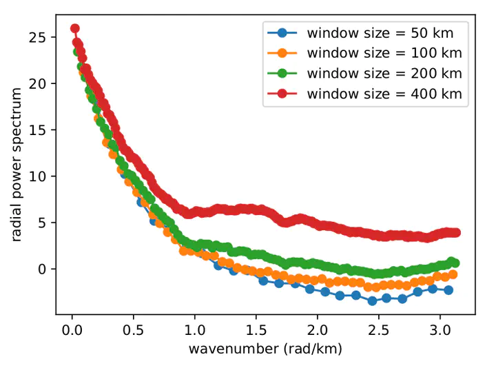 Radial power spectrum of the magnetic anomaly using different window sizes
Magnetic data is easy to come by on the surface of the Earth. It is relatively cheap to measure the magnetic anomaly using light aircrafts or drones, and susceptibility meters can be bundled along with gravity meters for additional prudence. Anomalies are assumed to reside on a horizontal surface at an elevation
As magnetite is the most magnetic mineral, the Curie depth is often interpreted to be the Curie point of magnetite - approximately 580C. Curie depth thus offers a very desirable isotherm in the lower crust.
Estimating the bottom of magnetic sources is usually accomplished by analysing the Fourier spectrum of magnetic anomalies. It’s computation is relatively simple:
Step-by-step
- Fast-Fourier transform (FFT) of the magnetic anomaly
- Shift the zero-frequency component to the center of the spectrum
- The gradient of the radial spectrum vs. wavenumbers of the power spectra obtains the Curie depth
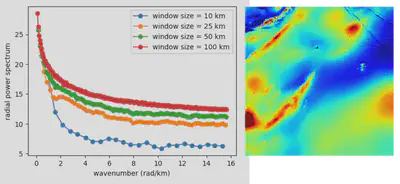
The caveat here is that the radial power spectra will vary significantly on the choice of window size and fractal parameters. A synthetic power spectrum was derived by Bouligand et al. (2009), eq. 4. We minimise the residual between the computed power spectrum,
Inverse problem
Gradient-based minimisation quickly converges to a model of minimum misfit between
At this point our inverse problem is somewhat ugly:
Curie depth computation involves two stages:
- Ensure there is no a priori information and commence with suitable starting values for
- Take the median and standard deviation of all parameters and add them as priors within the misfit function, then run the optimisation again.
Sensitivity analysis
A sensitivity analysis is essential to gauge the amount of uncertainty in a Curie depth determination, given the highly non-unique nature of this inverse problem. We randomly perturb each of
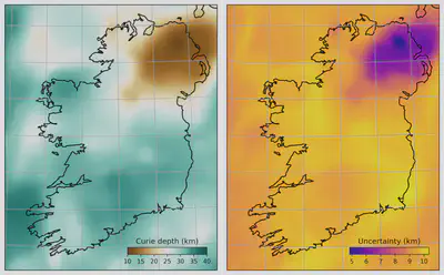
Above is the Curie depth we calculated across Ireland using the EMAG2 global magnetic anomaly compilation. Download PyCurious and try the code out for yourself.
Dr. Ben Mather
Research Fellow in Geophysics
My research interests include Bayesian inversion, Python programming and Geodynamics.